How to Use Microsoft Excel for Homeschool Lesson Planning [10 Tips]

Staying organized while homeschooling isn’t easy. In addition to covering all the essential subjects, you also have to adapt to your student’s individual learning pace, plus take care of all the nonacademic essentials such as keeping the home tidy and allowing kids to have time for social activities.

Organization is crucial because it facilitates the learning process for homeschoolers.

Excel is an excellent solution for homeschool lesson planning because it’s a readily available product that offers monthly plans for people who don’t want to commit to a software investment. Because it’s also very customizable, Excel suits households’ varying needs. You can use it while homeschooling one child or several.

There are specific things people can do to make Excel work best for them while lesson planning. You can dive into them by following the step-by-step instructions below.

1. Use Conditional Formatting to Color-Code Cells

It takes a long time to select Excel cells and format them individually. Luckily, Excel’s conditional formatting feature allows applying colors to blocks of cells.

Open an Excel worksheet and start by selecting the blocks of cells that require color. If selecting an entire row, click the top of the row, then CTRL + A.

Then, choose the Conditional Formatting button from the Excel options ribbon at the top of the screen.

From the drop-down menu, choose Highlight Cells Rules and select an option. For example, if you select Equal To and type “no” into the box and pick a color, all cells in the selected row containing the word no get filled with your chosen hue.

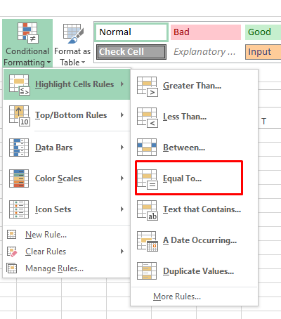
Try doing that to indicate chapters read, subjects covered and so on by creating a Done column where the input typed is either yes or no. Then, you can see at a glance what’s finished and what’s left to do.

2. Change the Widths of Columns

A default notebook page in Excel seemingly doesn’t offer ample room for taking notes or adding other specifics. However, you can quickly change the column widths so they provide more space for typing content that helps you keep track of educational necessities.

Just place your cursor to the left of the column you want to alter. Watch for it to change into an icon that looks like a double-headed arrow.

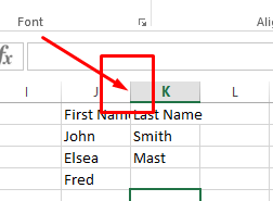
When you see it, click and drag until you achieve the desired width.

3. Create Sections for Each School Day

Breaking educational content down by day makes it simple to ensure you’re teaching enough material to reach end-of-the-year goals.

Split your Excel spreadsheet into sections that represent a school week to spread out the material, so you and your kids don’t get overwhelmed. The easiest way to do that is to download a free, preformatted spreadsheet tailored for lesson planning. After grabbing the file, you can customize it as desired.

4. Designate One Color for Each Core Subject

You can make the core subjects, such as math and reading, easily identifiable by assigning each one particular color. Choose pink for reading and blue for science, for example.

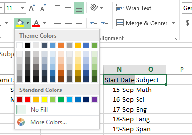
Do that by selecting a cell to fill with color, then finding the Excel icon in the menu bar that looks like a tilted bucket of paint. When you click on it, a menu appears so you can choose your preferred color.

5. Use Excel Rows to Make a Time-Based Schedule

One of the notable benefits of going paperless by using Excel for lesson planning is you won’t take up so much space with physical paperwork, which could result in less time spent tidying up students’ home work spaces.

Time spent is also a useful thing to document on an Excel learning plan. Use the left-side rows to make time-based cells for each lesson, such as 1:30-2:30, then enter the type of lesson taught to the right of the time. If needed, change the column width as instructed above. Place the cursor in a cell and click to start typing.

You can also use the drop-down font type and size buttons to customize the text typed into a cell. This is visible in the left corner of the screenshot above.

6. Create a Monthly Calendar in Excel

Many people don’t realize that Excel offers more than a typical spreadsheet. You can make a calendar in Excel and use it to get view of months at a time. Try that if you want a more traditional way to keep track of lessons that allows a broader overview.

Start by clicking the Developer tab in the Excel options ribbon. Then, choose Visual Basic.

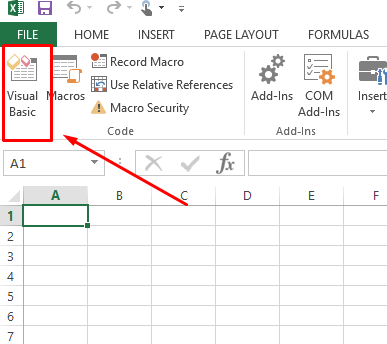
Then, from Excel’s Insert menu, choose Module. Copy the code listed here into the Module window. Click the File menu and choose Close and Return to Microsoft Excel. Next, select the Sheet1 tab along the left bottom side of the Excel window, seen in the above image. Go back to the Developer tab in the options ribbon and choose Macros. Finally, pick the CalendarMaker and click Run.

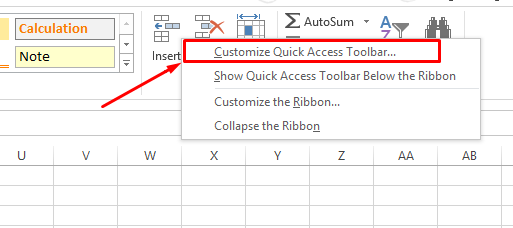
If you don’t see the Developer tab, right-click in any unoccupied area of the Excel ribbon and choose Customize the Ribbon.

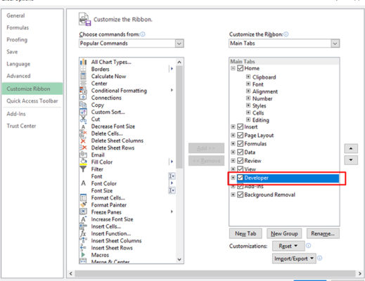
You’ll then see an options box containing all the possible additions for the ribbon. Pay attention to the Main Tabs section and look for Developer in that list. When you find it, check the box next to it to make the Developer tab show up in the Excel ribbon. Then, click OK.

7. Highlight School Holidays or Vacations

Many families choose to observe the local public school schedule, even when homeschooling.

Whether you make a calendar in Excel or keep the format as a spreadsheet, come up with an easily visible way that makes holidays and vacations stand out. You might use bold or italicized font, plus a different style than the rest of the sheet.

Consider filling all non-school days with black so you don’t get accidentally plan school activities during off-time.

8. Annotate Your Spreadsheets for Additional Context

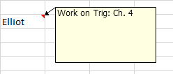
Excel makes it possible to insert annotations into particular cells. Doing that allows you to add details like student achievements or reasons for absences.

An annotated cell has a red indicator in the upper right corner.

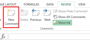
First, click the Review tab in the Excel options ribbon. Then, click the New Comment. Next, press Shift + F2. Right-click the cell that needs a comment, then choose Add Comment and type the content.

9. Make Lesson Plans Look More Exciting With Images

You can populate your Excel spreadsheets with images in about a minute.

Click Excel’s Insert tab first. Choose Illustrations, then Pictures. This will be in the Pictures tab in Excel 2013.

 

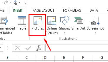
From there, a file dialogue box appears containing all the files on your computer. Select an image and click the dialogue box’s Insert button to add it into the spreadsheet. Grab and drag the corners of the spreadsheet to resize the image if needed.

Including pictures could help you give a lesson plan a seasonal theme or feature images that make you feel calm or inspired.

10.  Put a Graph or Chart Into Your Lesson Plan to Illustrate Statistics

You may want to indicate how many times your student received an A grade on a test or showed another sign of educational progress.

Excel allows inserting graphs or charts into spreadsheets, which could help you find areas of excellence or need for improvement. Simply go back to the Insert menu at the top of the Excel screen. Choose Charts from the options.

After that, the available chart styles appear, and you can pick one to insert into the spreadsheet.

All charts include sample data, but you can replace it with the statistics from your lesson plans by clicking on an area of the chart, deleting what’s there and putting in the correct information.

11. Use Flash Fill to Automate Data Entry

Excel’s Flash Fill feature automatically populates your cells with data if it senses a pattern in the things you type. It’s similar to the auto-correct feature on your phone and is available in Excel 2013 or later.

To activate it, go to the Data tab, then click the icon under the Data Tools section that looks like a spreadsheet with a lightning bolt in the corner.

In some cases, your button may not have the Flash Fill label, but it contains the lightning bolt icon. There’s also a drop-down menu to find a separate button in the Home page under the Fill menu.

 

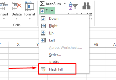
You can also activate Flash Fill by pressing CTRL+E instead of clicking the button, too. Bear in mind that this feature only works if you already have some data populating the fields. It needs to analyze existing data to try and find patterns.

A Note About Printing

When you choose Print from Excel’s file menu, it gives you numerous options, such as to only print the active sheets or to change the orientation.

For example, the Print Range drop-down menu offers ways to print full worksheets or only certain sections.

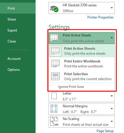
Becoming familiar with the printing options allows you to get the expected results without wasting paper or getting frustrated.

Less Stress, More Teaching

Excel is a powerful tool, but it can be overwhelming if you don’t know it well. These Excel tips take the stress out of lesson planning. They let you spend less time getting ready to teach and more time actually educating learners.

To make things even more straightforward, you can buy individual courses from K12 or consider enrolling students in a virtual school. Both those options allow you to support your child’s education at home while taking pressure off of you.